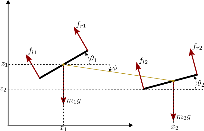
Dual pvtol, no load

• Generalized coordinates

\[q=\begin{pmatrix}x&z&\theta&\phi&\theta_2\end{pmatrix}^T\]

• Kinematic

\[\begin{cases} x_2 = x + l \cos{\phi} \\ z_2 = z + l \sin{\phi} \end{cases}\] \[\begin{cases} \dot{x}_2 = \dot{x} - l \dot{\phi} \sin{\phi} \\ \dot{z}_2 = \dot{z} + l \dot{\phi} \cos{\phi} \end{cases}\] \[\begin{cases} \ddot{x}_2 = \ddot{x} - l( \ddot{\phi} \sin{\phi} + \dot{\phi} \cos{\phi} ) \\ \ddot{z}_2 = \ddot{z} + l( \ddot{\phi} \cos{\phi} - \dot{\phi} \sin{\phi} ) \end{cases}\]

• Kinetic energy

\[T = \frac{1}{2} m_1 (\dot{x}^2+\dot{z}^2) + \frac{1}{2} J_1 \dot{\theta}^2 + \frac{1}{2} m_2 (\dot{x}_2^2+\dot{z}_2^2) + \frac{1}{2} J_2 \dot{\theta}_2^2\]

Introducing our generalized coordinates leads to

\[T = \frac{1}{2} \left(m_1+m_2\right) (\dot{x}^2+\dot{z}^2) + \frac{1}{2} J_1 \dot{\theta}^2 + \frac{1}{2} m_2 l\dot{\phi} \left(l\dot{\phi} - 2(\dot{x}\sin\phi-\dot{z}\cos\phi\right)+ \frac{1}{2} J_2 \dot{\theta}_2^2\]

• Potential energy

\[V = m_1 g z + m_2 g z_2\]

Introducing our generalized coordinates leads to

\[V = (m_1+m_2) g z + m_2 g l \sin{\phi}\]

Lagrangian

\[\mathcal{L} = T - V\]

• Partial derivatives

\[\begin{align*} \frac{\partial{\mathcal{L}}}{\partial{x}} &= 0 \\ \frac{\partial{\mathcal{L}}}{\partial{z}} &= -(m_1+m_2)g \\ \frac{\partial{\mathcal{L}}}{\partial{\theta}} &= 0 \\ \frac{\partial{\mathcal{L}}}{\partial{\phi}} &= -m_2l\left(\dot{\phi}(\dot{x}\cos\phi+\dot{z}\sin\phi) + g\cos\phi\right) \\ \frac{\partial{\mathcal{L}}}{\partial{\theta_2}} &= 0 \\ \frac{\partial{\mathcal{L}}}{\partial{\dot{x}}} &= \left(m_1+m_2\right)\dot{x} - m_2l\dot{\phi}\sin\phi \\ \frac{\partial{\mathcal{L}}}{\partial{\dot{z}}} &= \left(m_1+m_2\right)\dot{z} + m_2l\dot{\phi}\cos\phi \\ \frac{\partial{\mathcal{L}}}{\partial{\dot{\theta}}} &= J_1\dot{\theta} \\ \frac{\partial{\mathcal{L}}}{\partial{\dot{\phi}}} &= m_2l\left(-\dot{x}\sin\phi +z\cos\phi+l\dot{\phi}\right) \\ \frac{\partial{\mathcal{L}}}{\partial{\dot{\theta_2}}} &= J_2\dot{\theta} \end{align*}\]

Lagrange equations

1. \[\frac{d}{dt}\left( \frac{\partial{\mathcal{L}}}{\partial{\dot{x}}} \right) - \frac{\partial{\mathcal{L}}}{\partial{x}} = F_x\]

\[\left( m_1+m_2 \right) \ddot{x} - m_2l \left( \ddot{\phi}\sin\phi + \dot{\phi}^2\cos\phi \right) = -(f_l+f_r)\sin\theta - (f_{l2}+f_{r2})\sin\theta_2\]

2. \[\frac{d}{dt}\left( \frac{\partial{\mathcal{L}}}{\partial{\dot{z}}} \right) - \frac{\partial{\mathcal{L}}}{\partial{z}} = F_z\]

\[\left( m_1+m_2 \right) (\ddot{z}+g) + m_2l \left( \ddot{\phi}\cos\phi - \dot{\phi}^2\sin\phi \right) = (f_l+f_r)\cos\theta + (f_{l2}+f_{r2})\cos\theta_2\]

3. \[\frac{d}{dt}\left( \frac{\partial{\mathcal{L}}}{\partial{\dot{\theta}}} \right) - \frac{\partial{\mathcal{L}}}{\partial{\theta}} = M_\theta\]

\[J_1 \ddot{\theta} = d_1 (-f_l+f_r)\]

4. \[\frac{d}{dt}\left( \frac{\partial{\mathcal{L}}}{\partial{\dot{\theta_2}}} \right) - \frac{\partial{\mathcal{L}}}{\partial{\theta_2}} = M_{\theta_2}\]

\[J_2 \ddot{\theta} = d_2 (-f_{l2}+f_{r2})\]

5. \[\frac{d}{dt}\left( \frac{\partial{\mathcal{L}}}{\partial{\dot{\phi}}} \right) - \frac{\partial{\mathcal{L}}}{\partial{\phi}} = M_\phi\]

\[l \ddot{\phi} - \sin\phi \ddot{x} + \cos \phi \ddot{z} = -\cos\phi g + \cos(\phi-\theta_2) \frac{f_{l2}+f_{r2}}{m_2}\]