\(\newcommand{\ddt}[2]{#1^{(#2)}}\)
1: Model
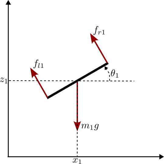
Applying Newton’s second law to our vehicle in ground frame, we get
\[\begin{align*} m\ddot{x} &= -(f_l+f_r)\sin(\theta) \\ m\ddot{z} &= -mg + (f_l+f_r)\cos(\theta) \\ J\ddot{\theta} &= d(-f_l+f_r) \end{align*}\]- Generalized coordinates
- Kinetic energy
- Potential energy
- Lagrangian
Partial derivatives
\[\begin{cases} \frac{\partial{L}}{\partial{x}} = 0 \\ \frac{\partial{L}}{\partial{z}} = - m g\\ \frac{\partial{L}}{\partial{\theta}} = 0 \\ \end{cases} \quad \begin{cases} \frac{\partial{L}}{\partial{\dot{x}}} = m\dot{x} \\ \frac{\partial{L}}{\partial{\dot{z}}} = m\dot{z} \\ \frac{\partial{L}}{\partial{\dot{\theta}}} = J \dot{\theta} \end{cases}\]Lagrange equations
*
\[\frac{d}{dt}\left( \frac{\partial{L}}{\partial{\dot{x}}} \right) - \frac{\partial{L}}{\partial{x}} = F_x\] \[m\ddot{x} = -(f_l+f_r) \sin{\theta}\]*
\[\frac{d}{dt}\left( \frac{\partial{L}}{\partial{\dot{z}}} \right) - \frac{\partial{L}}{\partial{z}} = F_z\] \[m\ddot{z} + mg = (f_l+f_r) \cos{\theta}\]*
\[\frac{d}{dt}\left( \frac{\partial{L}}{\partial{\dot{\theta}}} \right) - \frac{\partial{L}}{\partial{\theta}} = M_{\theta}\] \[J\ddot{\theta} = d \left(-f_l+f_r \right)\]State Space Representation
Using \(X = \begin{pmatrix}x&z&\theta&\dot{x}&\dot{z}&\dot{\theta}\end{pmatrix}^T\) as state and \(U = \begin{pmatrix}f_l & f_r \end{pmatrix}^T\) as input, a state space representation can be obtained as:
\[\begin{equation} \dot{X} = f(X,U) = \begin{pmatrix} \dot{x} \\ \dot{z} \\ \dot{\theta} \\ -\frac{1}{m} \sin{\theta} \left( f_l+f_r \right) \\ -g + \frac{1}{m} \cos{\theta} \left( f_l+f_r \right)\\ \frac{d}{J} \left( -f_l+f_r \right) \end{pmatrix} \end{equation}\]The following input variable change: \(U' = \begin{pmatrix}u_t\\u_d\end{pmatrix} = \begin{pmatrix}\frac{1}{m}(f_l+f_r) \\ \frac{d}{J}(-f_l+f_r)\end{pmatrix}\) leads to the simplified state space representation
\[\begin{equation} \dot{X} = f'(X,U') = \begin{pmatrix} \dot{x} \\ \dot{z} \\ \dot{\theta} \\ -\sin{\theta}. u_t \\ -g + \cos{\theta}. u_t\\ u_d \end{pmatrix} \end{equation}\]2: Control
2.1: Full State Feedback Regulation
Here we stabilize the vehicle around an equilibrium \(X_e\), \(U_e\)
\(X_e = \begin{pmatrix}x_e&z_e&0&0&0&0\end{pmatrix}^T\) \(U_e = \begin{pmatrix}mg/2&mg/2\end{pmatrix}^T\)
Noting \(\delta X = X-X_e\) and \(\delta U = U-U_e\), we obtain the linearized model as
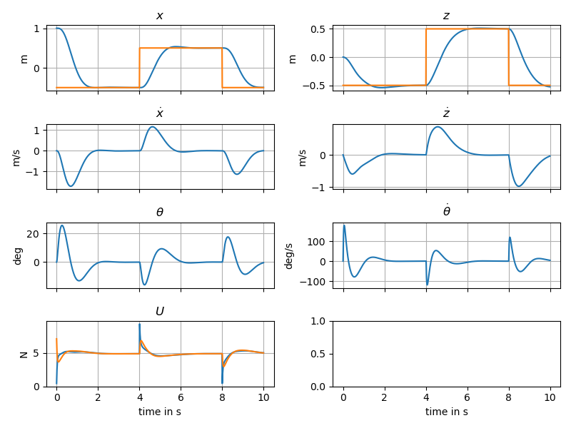
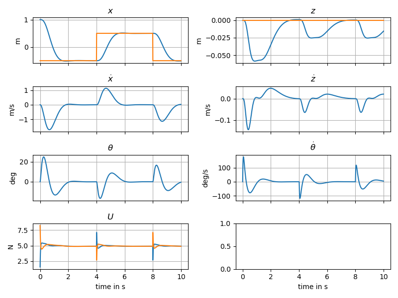
\[\dot{\delta X} = \begin{pmatrix}0&0&0&1&0&0\\0&0&0&0&1&0\\0&0&0&0&0&1\\ 0&0&-g&0&0&0\\0&0&0&0&0&0\\0&0&0&0&0&0\end{pmatrix}\delta X + \begin{pmatrix}0&0\\0&0\\0&0\\0&0\\1/m&1/m\\-d/J&d/J\end{pmatrix} \delta U\]The linearized system is fully controllable. the non-linear system can hence be stabilized using a state feeback \(U = U_e - K \delta X\) In the example a gain is computed using LQR, leading to the following simulations;
TODO: linear invert control
2.2: Trajectory tracking
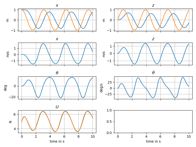
In the previous part, we notice the regulation showing its limit on the circle example. In order to improve trajectory following, we will improve the open-loop part of our controller.
The differential flatness property of the vehicle can be leveraged in order to follow a dynamic trajectory \(Yr(t)=\begin{pmatrix}x_r(t), y_r(t)\end{pmatrix}\)
Given a sufficiently smooth trajectory, it is possible to obtain the state vector \(X_r(t)\) and the input \(U_r(t)\) from a number of time derivatives of the output \(Y_r\)
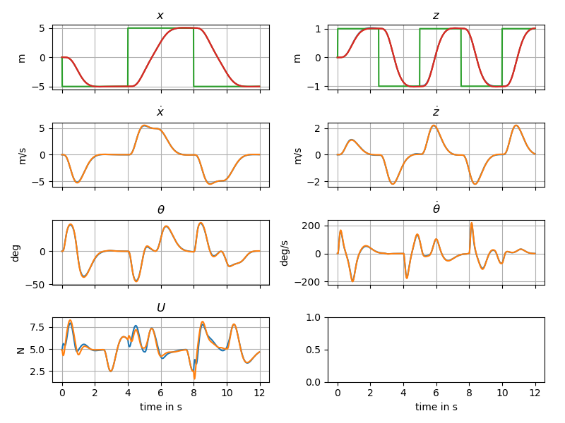
\[X_r = \begin{pmatrix} \ddt{x}{0} \\ \ddt{z}{0} \\ -\arctan\frac{\ddt{x}{2}}{\ddt{z}{2}+g} \\ \ddt{x}{1} \\ \ddt{z}{1} \\ -\frac{\left(\ddt{z}{2}+g\right)\ddt{x}{3} - \ddt{x}{2}\ddt{z}{3}} {\left(\ddt{z}{2}+g\right)^2 + \left(\ddt{x}{2}\right)^2} \end{pmatrix}\] \[U_r = \begin{pmatrix} \sqrt{\left(\ddt{x}{2}\right)^2 + \left(\ddt{z}{2}+g\right)^2}\\ \frac{\left[\ddt{x}{4}(\ddt{z}{2}+g)-\ddt{z}{4}\ddt{x}{2}\right] \left[(\ddt{z}{2}+g)^2 + (\ddt{x}{2})^2\right] - \left[2(\ddt{z}{2}+g)\ddt{z}{3} + 2\ddt{x}{2}\ddt{x}{3}\right] \left[\ddt{x}{3}(\ddt{z}{2}+g) - \ddt{z}{3}\ddt{x}{2}\right]} {\left(\left(\ddt{z}{2}+g\right)^2 + \left(\ddt{x}{2}\right)^2\right)^2}\\ \end{pmatrix}\]The controller \(U = U_r + K(X-X_r)\) can be shown to achieve perfect trajectory traking while providing asymptotically stable error rejection.
2.3: Reference Model
The smooth trajectory can be generated from a reference model like is done in Admittance Control for Physical Human-Quadrocopter Interaction.
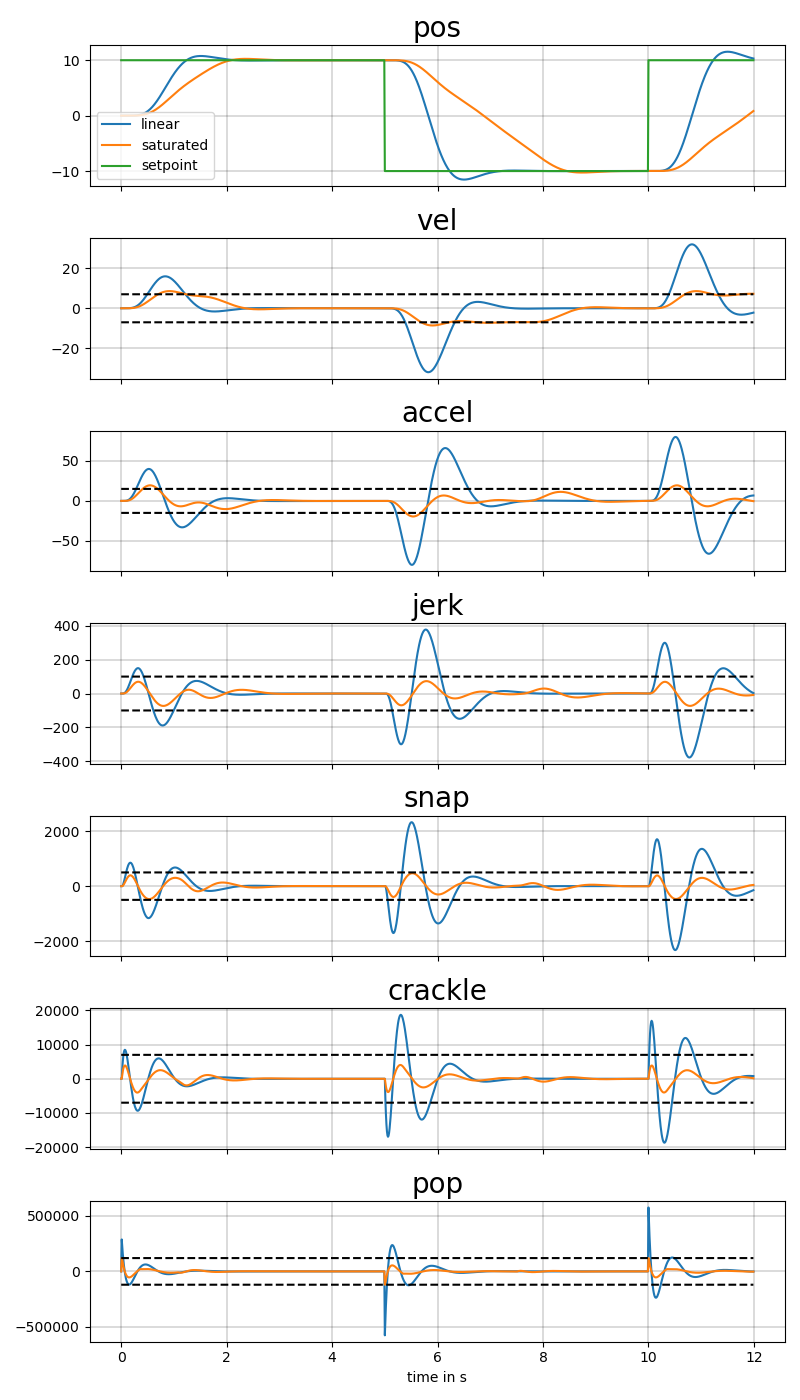
Adaptive Control with a Nested Saturation Reference Model describes a saturated pseudo-linear model which is implemented here. Saturations can can be disabled and the model reverted to a classic linear model.