We will start by deriving a dynamic model for the PVTOL with pole system.

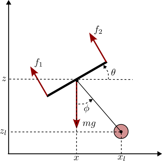
It can be seen that the vector \(q=\begin{pmatrix}x&z&\theta&\phi\end{pmatrix}^T\) can be used a generalized coordinates as it uniquely describes the configuration of the system.

Kinematic

Assumingt that the pole is constrained to pivot at the center of the PVTOL, the position of the center of mass of the pole is then given by:

\[\begin{cases} x_p = x - l \sin{\phi} \\ z_p = z + l \cos{\phi} \end{cases}\]

Computing the time derivative of the above equation, we get the velocity of the pole’s center of mass as:

\[\begin{cases} \dot{x}_p = \dot{x} - l \dot{\phi} \cos{\phi} \\ \dot{z}_p = \dot{z} - l \dot{\phi} \sin{\phi} \end{cases}\]

Noting \(v^2=\dot{x}^2+\dot{z}^2\) and \(v_p^2=\dot{x}_p^2+\dot{z}_p^2\), the relationship between the pvtol and pole centers of mass velocities is expressed as:

\[v_p^2 = \dot{x}^2 + \dot{z}^2 + l^2\dot{\phi}^2 -2l\dot{\phi}\left( \dot{x}\cos{\phi}+\dot{z}\sin{\phi}\right)\] \[v_p^2 = v^2 + l^2\dot{\phi}^2 -2l\dot{\phi}\left( \dot{x}\cos{\phi}+\dot{z}\sin{\phi}\right)\]

Energy

	Kinetic Energy	Potential Energy
pvtol	$$ T_v = \frac{1}{2} Mv^2 + \frac{1}{2} J \dot{\theta}^2$$	$$ V_v = Mgz$$
pole	$$ T_p = \frac{1}{2} mv_p^2 + \frac{1}{2} j \dot{\phi}^2$$	$$ V_p = mgz_p$$

Lagrangian

\[\mathscr{L} = T - V\] \[\mathscr{L} = \frac{1}{2}Mv^2 + \frac{1}{2} J \dot{\theta}^2 +\frac{1}{2}mv_p^2 + \frac{1}{2} j \dot{\phi}^2 - Mgz - mgz_p\]

Expanding with state variables, we get:

\[\begin{multline} \mathscr{L} = \frac{1}{2} \left( M+m \right) \left( \dot{x}^2 + \dot{z}^2 \right) + \frac{1}{2} J \dot{\theta}^2 + \frac{1}{2} j \dot{\phi}^2 \\ + \frac{1}{2}m\left( l^2\dot{\phi}^2 -2l\dot{\phi}\left( \dot{x}\cos{\phi}+\dot{z}\sin{\phi}\right) \right) - \left( M+m \right) g z - mgl \cos{\phi} \end{multline}\]

Partial derivatives of the Lagrangian with respect to the state vector components are:

\[\begin{cases} \frac{\partial{\mathscr{L}}}{\partial{x}} = 0 \\ \frac{\partial{\mathscr{L}}}{\partial{z}} = - \left( M+m \right) g\\ \frac{\partial{\mathscr{L}}}{\partial{\theta}} = 0 \\ \frac{\partial{\mathscr{L}}}{\partial{\phi}} = ml \left( \dot{\phi} \left( \dot{x}\sin{\phi} - \dot{z}\cos{\phi}\right) + g \sin{\phi}\right)\\ \frac{\partial{\mathscr{L}}}{\partial{\dot{x}}} = \left( M+m \right) \dot{x} - ml\dot{\phi}\cos{\phi}\\ \frac{\partial{\mathscr{L}}}{\partial{\dot{z}}} = \left( M+m \right) \dot{z} - ml\dot{\phi}\sin{\phi}\\ \frac{\partial{\mathscr{L}}}{\partial{\dot{\theta}}} = J \dot{\theta}\\ \frac{\partial{\mathscr{L}}}{\partial{\dot{\phi}}} = j \dot{\phi} + ml \left( l\dot{\phi} - \left( \dot{x}\cos{\phi}+\dot{z}\sin{\phi} \right)\right)\\ \end{cases}\]

Lagrange Equations

*

\[\frac{d}{dt}\left( \frac{\partial{\mathscr{L}}}{\partial{\dot{x}}} \right) - \frac{\partial{\mathscr{L}}}{\partial{x}} = F_x\] \[\left( M+m \right) \ddot{x} - ml \left( \ddot{\phi} \cos{\phi} - \dot{\phi}^2\sin{\phi}\right) = -(f_1+f_2) \sin{\theta}\]

*

\[\frac{d}{dt}\left( \frac{\partial{\mathscr{L}}}{\partial{\dot{z}}} \right) - \frac{\partial{\mathscr{L}}}{\partial{z}} = F_z\] \[\left( M+m \right) \ddot{z} - ml \left( \ddot{\phi} \sin{\phi} + \dot{\phi}^2\cos{\phi}\right) + \left( M+m \right) g = (f_1+f_2) \cos{\theta}\]

*

\[\frac{d}{dt}\left( \frac{\partial{\mathscr{L}}}{\partial{\dot{\theta}}} \right) - \frac{\partial{\mathscr{L}}}{\partial{\theta}} = M_{\theta}\] \[J\ddot{\theta} = L \left( -f_1+f_2 \right)\]

*

\[\frac{d}{dt}\left( \frac{\partial{\mathscr{L}}}{\partial{\dot{\phi}}} \right) - \frac{\partial{\mathscr{L}}}{\partial{\phi}} = 0\] \[(j+ml^2)\ddot{\phi} - ml \left( \ddot{x}\cos{\phi} + (\ddot{z}+g)\sin{\phi} \right) = 0\]

State Space Representation

We have now obtained 4 coupled ODEs that needs to be uncoupled to obtain a SSR.

\[\begin{cases} \ddot{x} - \frac{ml}{M+m} \cos{\phi} \ddot{\phi} = - \frac{ml}{M+m} \sin{\phi} \dot{\phi}^2 - \frac{1}{M+m} \sin{\theta} (f_1 +f_2) \\ \ddot{z} - \frac{ml}{M+m} \sin{\phi} \ddot{\phi} = \frac{ml}{M+m} \cos{\phi} \dot{\phi}^2 -g + \frac{1}{M+m} \cos{\theta} (f_1 +f_2) \\ \ddot{\theta} = \frac{L}{J}(-f_1+f_2) \\ \ddot{\phi} -\frac{ml}{j+ml^2}\left( \ddot{x} \cos{\phi} + (\ddot{z} + g) \sin{\phi} \right) = 0 \end{cases}\]

The above can be matricially rewritten as a linear system: \(\begin{pmatrix} 1 & 0 & 0 & a \\ 0 & 1 & 0 & b \\ 0 & 0 & 1 & 0 \\ c & d & 0 & 1 \end{pmatrix} \begin{pmatrix} \ddot{x}\\ \ddot{z} \\ \ddot{\theta} \\ \ddot{\phi} \end{pmatrix} = \begin{pmatrix} e \\ f \\ g \\ h \end{pmatrix}\)

The system has full rank ( \(det(A) = 1\) ).